Introduction
Adversarial examples are a large obstacle for a variety of machine learning systems to overcome. Their existence shows the tendency of models to rely on unreliable features to maximize performance, which if perturbed, can cause misclassifications with potentially catastrophic consequences. The informal definition of an adversarial example is an input that has been modified in a way that is imperceptible to humans, but is misclassified by a machine learning system whereas the original input was correctly classified. The below figure illustrates the the concept
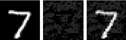 Original image (left), adversarial noise (middle), perturbed image incorrectly classified as a 2 (right)
The formal definition of an adversarial example is as follows
\[\begin{align*} x_{\mathrm{adv}} = \max_{\delta} \mathcal{L}(\mathbf{f}, x_{\mathrm{orig}}, y) \\ \mathrm{such \: that\:\:} ||\delta||_{p} \leq \epsilon \\ \mathrm{and\:\:} x_{orig} + \delta \in [0, 1]^{D} \end{align*}\]where \(\mathcal{L}\) is the loss function we are trying to maximize, \(x_{orig}\) is the original image, \(\delta\) is the perturbation, \(y\) is the ground truth label, and \(\epsilon\) is chosen to ensure that the perturbed image does not look too noisy, and such that it still looks like an image of the original class to humans. Several attacks, such as FGS, IGS, and PGD use the L-\(\infty\) norm to constrain the distance between the perturbed and original image. In this post, we will explore the difficulties of choosing \(\epsilon\) for the MNIST dataset. We will also look at recent techniques of generating adversarial examples do not rely on perturbing some original image and question if such generated images actually satisfy the definition of an adversarial example.
MNIST Distance Analysis
Let’s begin with a simple analysis of the average distance between images of the same class, and between images of different classes. Perhaps these distances can assist in choosing \(\epsilon\) in a more quantitative and less subjective way. A link to the Jupyter notebook for this analysis can be found at the end of this post.
We sample 100 random images from each class, and compute the average pairwise distance between images under various norms. Just the L-2 norm is shown here to avoid clutter, and also because the L-\(\infty\) norm heatmap simply has a 1 in every cell and is not informative.
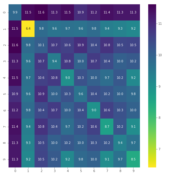 L-2 Norm Training Set Distances
A reasonable assumption to make is that the diagonal elements of this heatmap (within-class distances) should be lower than the off-diagonal elements in the same row/column (between-class distances). However, this is not the case as is seen above for 2s which are closer to 1s, and 8s which are also closer to 1s. This is a surprise at first, but it just indicates that the variation in style for a given digit might cause more pixel differences than switching between digits. One can consider this to be an artefact of how for every digit, there is a set of invariant pixels that does not change for different images of that digit, and when the invariant sets of two digits have high overlap, unexpected results like those above can occur.
Choosing \(\epsilon\)
What does this all mean when it comes to choosing \(\epsilon\)? The most common value of \(\epsilon\) when using the L-\(\infty\) norm is 0.3, and a high value for the L-2 norm is 4.5 (Madry et al.). If we consider the most extreme value of \(\epsilon\)=1.0 for the L-\(\infty\) norm, we would have no control over the ground truth class of the perturbed image, and might end up generating an image that looks like a different class to both humans and our image classification model. This would also allow us to arbitrarily interpolate between train and test set images \(x' = rx_{\mathrm{train}} * (1-r)x_{\mathrm{test}}\), and if our model happens to incorrectly classify \(x_{\mathrm{test}}\), then it would be flagged as adversarial. So there are multiple conditions to enforce here.
- We want the set of allowable perturbations to be imperceptible to humans when comparing an original image \(x\) and its perturbed version \(x'\) side by side
- We want it to be impossible for a perturbation to result in interpolating between images of the same digit. Otherwise, this can confound adversarial robustness with generalization performance. For a given digit \(d\), and test set images \(x_{\mathrm{correct}}\) and \(x_{\mathrm{false}}\) which are respectively correctly and incorrectly classified by our model, a trivial adversarial attack would be to transform \(x_{\mathrm{correct}}\) into \(x_{\mathrm{false}}\)
Depending on the observer, (1) will usually imply (2). \(\epsilon\)=0.3 certainly satisfies (2) since all images have an L-\(\infty\) distance close to 1.0. Let’s look at what happens if we generate images that are combinations of 2 classes as follows
\[\begin{equation*} x_{\mathrm{combined}} = x_{0} + \epsilon * \mathrm{sign} (x_{1}) \end{equation*}\]This bounds the L-\(\infty\) distance between the original image and the crafted image to \(\epsilon\), but any human observer can easily tell the difference between two images like those below
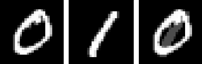 Crafted image within ε=0.3 L-inf distance of original
It’s quite obvious that there is something off about the rightmost image. In fact, without being told that this is an image that is a combination of a 0 and 1, some might say it’s just an abstract symbol. So with a simple example, we’ve shown that \(\epsilon\)=0.3 violates condition (1). Even a smaller value such as \(\epsilon\)=0.2 gives similar results. MNIST allows for easy identification of perturbed pixels. In many cases it is trivial to create a detection mechanism for adversarial examples by simply checking if a modification was made to background pixels. If attacks are made aware of this detection mechanism though, they can bypass it (Carlini and Wagner). How can we then choose \(\epsilon\)?
There is a case to be made for not using the same \(\epsilon\) for every image. For some classes, it is much easier to tell if pixels have been changed within the bounding box of the digit itself, like in the example above. \(\epsilon\) should probably be set to a smaller value for such classes. Additionally, typical norms like L-2 or L-\(\infty\) have no notion of semantic similarity when they are used to compute distances in image space. If they were able to give semantic similarities between images in input space, then it would be possible to construct a simple KNN image classifier and do away with the advances in convolutional neural networks over the past 7 years. A possible solution to this issue is to use techniques from metric learning. By learning embeddings where L-2 or L-\(\infty\) distance between such embeddings contains a notion of semantic similarity, then we could tune \(\epsilon\) in this space rather than input space. One such technique is called triplet networks. Triplet networks function by passing 3 images at once to the same embedding network in parallel. An anchor of class \(y\) is passed through, along with a positive example (+) of the same class, and a negative example (-) of a different class \(y'\). The loss function ensures that distance between the anchor and the positive example is at least \(\alpha\) smaller than the distance between the anchor and the negative example.
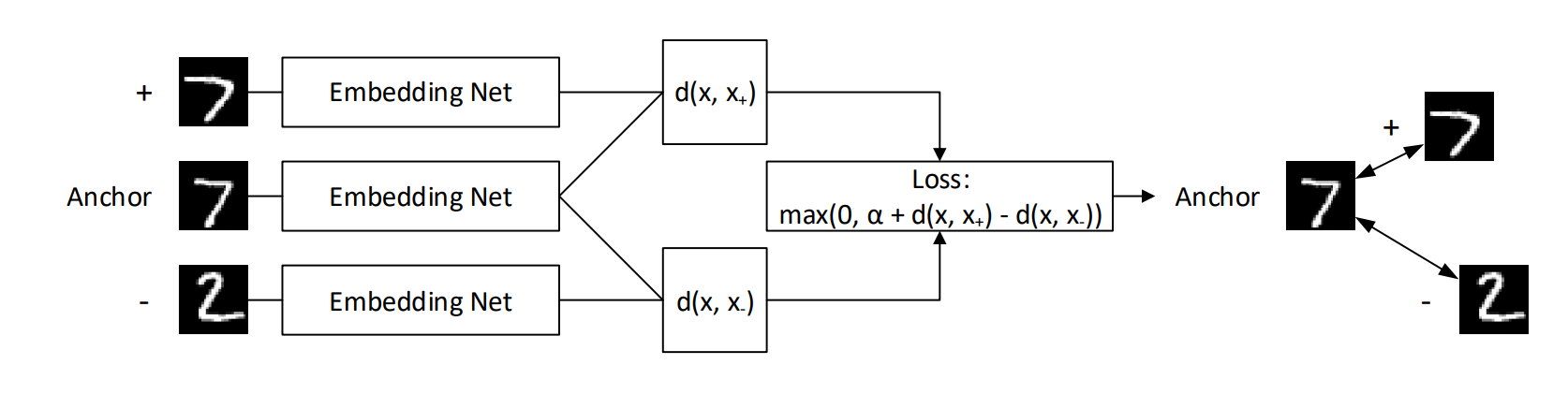 Illustration of a what a triplet network does
Using a metric learning technique like triplet networks would still require manual experimenter verification to ensure that ε is not chosen large enough that it allows for changes in class. Furthermore, we would have to take into account condition (2) which says that we shouldn’t be able to jump from one image in our dataset to another of the same class using perturbations. An attack like PGD iteratively moves in the direction of the gradient of the loss function to increase the loss, and then projects the resulting image onto a subspace of inputs satisfying distance constraints from the original image. Instead of doing this projection in input space, it would be done in embedding space by our metric learning algorithm of choice.
Generative Adversarial Examples
A very cool paper (Song et al.) introduces a new way of creating adversarial examples. Rather than perturbing some already existing image using adversarially crafted noise, the authors opt to use a GAN to generate images from scratch that are likely to fool the model being attacked. Specifically, they use an auxiliary classifier GAN (AC-GAN) which is able to condition on image class in order to have control over what kind of image is being generated. This results in “unrestricted adversarial examples” since there is no distance to constrain because the images are generated from scratch. However, this does not satisfy either criteria (1) or (2) mentioned previously. While their technique is very useful, and allows for model debugging as well as data augmentation by generating new images on which the model fails, the analysis treats generalization performance and adversarial robustness as the same thing. In order to properly analyze model robustness, we need to be able to disentangle the two metrics of generalization performance and adversarial robustness, since they are at odds with each other (Tsipras et al.). So while it may be tempting to move away from perturbation-based definitions of adversarial examples, for now they are the only method that allows for studying adversarial robustness in an isolated, non-confounded fashion.
Conclusion
The current definition of adversarial examples is slightly flawed for a dataset such as MNIST, though it makes much more sense for something like ImageNet where the perturbations are much more difficult to notice, and do not end up making images look like strange combinations of classes. Using the same threshold \(\epsilon\) for every image or class can be a punishing requirement as it is easier to detect noise for images of a particular class. Images are a type of data that is naturally easy for humans to analyze and judge whether or not something fishy is going on. However, many domains exist where data comes in the form of abstract vectors of numbers that are very difficult to understand and visualize. Definining what is adversarial in such domains might be beyond the limits of our imagination since we cannot understand the original data to begin with. In such cases, quantitative methods of coming up with \(\epsilon\) are a must.
I hope you’ve enjoyed this post, and let me know what other topics you’d like to see covered in future posts.