Introduction
For the past couple of years, researchers and companies have been trying to make deep learning more accessible to non-experts by providing access to pre-trained computer vision or machine translation models. Using a pre-trained model for another task is known as transfer learning, but it still requires sufficient expertise to fine-tune the model on another dataset. Fully automating this procedure allows even more users to benefit from the great progress that has been made in ML to date.
This is called AutoML, and it can cover many parts of predictive modelling such as architecture search and hyperparameter optimization. In this post, I focus on the former, as there has been a recent explosion of methods that search for the “best” architecture for a given dataset. The results presented are based on joint work with Jonathan Lorraine.
The Importance of Neural Network Architecture
As a side note, keep in mind that a neural network with just a single hidden layer and non-linear activation function is able to represent any function possible, provided that there are sufficient neurons in that layer (UAT). However, such a simple architecture, though it is theoretically able to learn any function, does not represent the hierarchical processing that occurs in the human visual cortex. The architecture of a neural network gives it an inductive bias, and shallow, wide networks that do not use convolutions are significantly worse at image classification tasks than deep, convolutional networks. Thus, in order for neural networks to generalize and not overfit the training dataset, it’s important to find architectures with the right inductive bias (regardless if those architectures are inspired by the brain or not).
Neural Architecture Search (NAS) Overview
NAS was an inspiring work out of Google that lead to several follow up works such as ENAS, PNAS, and DARTS. It involves training a recurrent neural network (RNN) controller using reinforcement learning (RL) to automatically generate architectures. These architectures then have their weights trained and are evaluated on a validation set. Their performance on the validation set is the reward signal for the controller which then increases its probability of generating architectures that have done well, and decreases the probability of generating architectures that have done poorly. For non-technical readers, this essentially takes the process of a human manually tweaking a neural network and learning what works well, and automating it. The idea of automatically creating NN architectures was not coined by NAS, as other approaches using methods such as genetic algorithms existed long before, but NAS effectively used RL to efficiently search a space that is prohibitively large to search exhastively. Below, the components of NAS are analyzed in a bit more depth, before I go on to discuss the limitations of the method as well as its more efficient successor ENAS, as well as an interesting failure mode. The next 2 subsections are best understood while comparing the text again the below figure showing how architectures are sampled and trained:

LSTM Controller
The controller generates architectures by making a series of choices for a pre-defined amount of time steps. For example, when generating a convolutional architecture, the controller begins by only creating architectures with 6 layers in them. For each layer, just 4 deicisions are made by the controller: filter height, filter width, number of filters, and stride (so 24 time steps). Assuming that the first layer is numbered 0, then the decisions \(C\) at a particular layer \(l\) are sampled as :
- Filter height is \(C_{l, h} \sim p_{l \times 4}\)
- Filter width is \(C_{l, w} \sim p_{l \times 4 + 1}\)
- Number of filters is \(C_{l, f} \sim p_{l \times 4 + 2}\)
- Stride is \(C_{l, s} \sim p_{l \times 4 + 3}\)
Note that the probability distribution at time step \(t\), \(p_{t} = f_{t}(h_{t})\) is just a linear function of the hidden state at that time step, followed by a softmax. Since the controller is an LSTM, its hidden state at the initial time step \(h_0 = [0, 0, ..., 0]^{\top}\) is set to a vector of all 0s. Each sampled decision has a preset group of values, such as [24, 36, 48, 64] for number of filters (looks like a probabilitic grid search). Eventually, the number of layers is increased, hence the need for dynamic computation that is offered by LSTMs. The hope is that the hidden state of the LSTM will remember past choices and bias the probability distributions of future time steps to take these choices into account.
Training Sampled Architectures
After a given architecture has been created, it is then trained for a limited number of epochs (50), and the validation accuracy \(\mathrm{Acc}_{v}\) is observed. Interestingly, a bit of mysterious reward shaping is involved as the maximum validation accuracy observed in the last 5 epochs is then cubed and taken to be the reward that is used to update the controller’s parameters using policy gradient:
\[\begin{equation*} R = \max\limits_{t \in \{46, ... 50\}} (\mathrm{Acc}_{v}^{(t)})^{3} \end{equation*}\]An important point to note for when I discuss ENAS later is that the weights of the trained architecture are then thrown away, and every time an architecture is sampled, they are randomly initialized. Since the architecture choices are so simple, a record of all the architectures that have been sampled, along with their validation accuracy is kept.
Choosing the Best Architecture
The best performing architecture observed during the training of the controller is taken, and a grid search is performed over some basic hyperparameters such a learning rate and weight decay in order to achieve near STOTA performance.
Efficient Neural Architecture Search (ENAS) Overview
The reason why NAS is not used by everyone, from deep learning experts to laymen, is due to its prohibitively expensive computational complexity. In fact, it requires ~32,000 GPU hours which makes one wonder why not hire an expert to design an architecture rather than invest so many resources in automatically searching for one. ENAS was created to address this very issue.
Weight Sharing
Instead of throwing away the weights learned for all the architectures that are sampled over the course of training, ENAS uses a pool of shared parameters which are continually updated. This means that by the time architecture 100 is sampled, it is initialized with weights that already provide reasonable accuracy, especially compared to random weights. This decreases the GPU hours required to find an architecture with excellent performance from 32,000 to ~50!
This is best understood with a figure as below. Recall that in the NAS example, I showed how an entire CNN architecture is created. Here, I will focus on a recurrent cell. A cell in the context of ENAS is essentially just a directed acyclic graph (DAG). The number of nodes in the DAG is specified beforehand, so just the connections are to be learned. The DAG can be thought of as a computation graph with edges representing matrix multiplications that transmit information from one node to another, and nodes representing different “hidden states”.
The DAG is constructed by choosing for each node:
- The activation function to use at that node, i.e. [tanh, sigmoid, ReLU]
- The previous node to connect the current node to, i.e. at node 4 the possible choices are [1,2,3]
The sampled DAG in the below figure is shown by the red arrows. The remaining blue arrows are not part of the sampled architecture, but just show some of the other connections that are possible when creating a DAG with 5 nodes in it. Blue nodes that are not filled in represent internal nodes, and oranges nodes represent leaf nodes. The leaf nodes have their outputs combined by averaging (or potentially some other mechanism), and this is taken to be the hidden state of the entire reccurent cell at the current time step \(h_t\). Black arrows represent hardcoded connections (i.e. there is no choice to be made here). For example, the cell always takes as input both the features at the current time step \(x_t\) and the hidden state of the cell at the previous time step \(h_{t-1}\).

Since there is a matrix associated with every edge in the DAG, the pool of shared parameters is just the set of all these matrices.
Why These Methods Do So Well?
Although the architectures (along with their learned weights) provided by NAS or ENAS give excpetional performance on image classification and language modelling tasks, it is not clear that this is due to the search method.
Ground Truth for Architecture Search
First of all, it is impossible to know the best architecture for a given dataset is without training every possbile one, and performing an extensive hyperparameter search for each architecture. This makes it difficult to say if the controller is actually exploring the space of possible architectures effectively, or if it’s simply recreating past architectures that have provided high validation accuracy. There is an entropy parameter which makes the probability distributions output by the controller at each time step be more uniform, thereby increasing exploration, but that exploration is essentially random, or it favors making slight changes to architectures that have already been deemed to be the best. This might not be an issue if all we care about is reaching some level of accuracy, but perhaps there is another explanation for the good performance.
Who Decides the Search Space?
The decisions made by the controller at each time step are extremely limited. They amount to choosing from a set of options that have already been deemed to work quite well for recurrent or convolutional architectures in the past. For example, the options for filter width are [1, 3, 5, 7] which are standard values that have been used in models like ResNets or DenseNets. Thus, the search space itself is biased in such a way that it is quite difficult to sample architectures that do badly. Obviously having more fine-grained choices increases the sample complexity of the search algorithm, but if we truly believe in the search algorithm’s effectiveness, we would not limit it to using values that we as humans have deemed to be effective since that might prevent the discovery of more effective architectures.
Comparison to Random Search
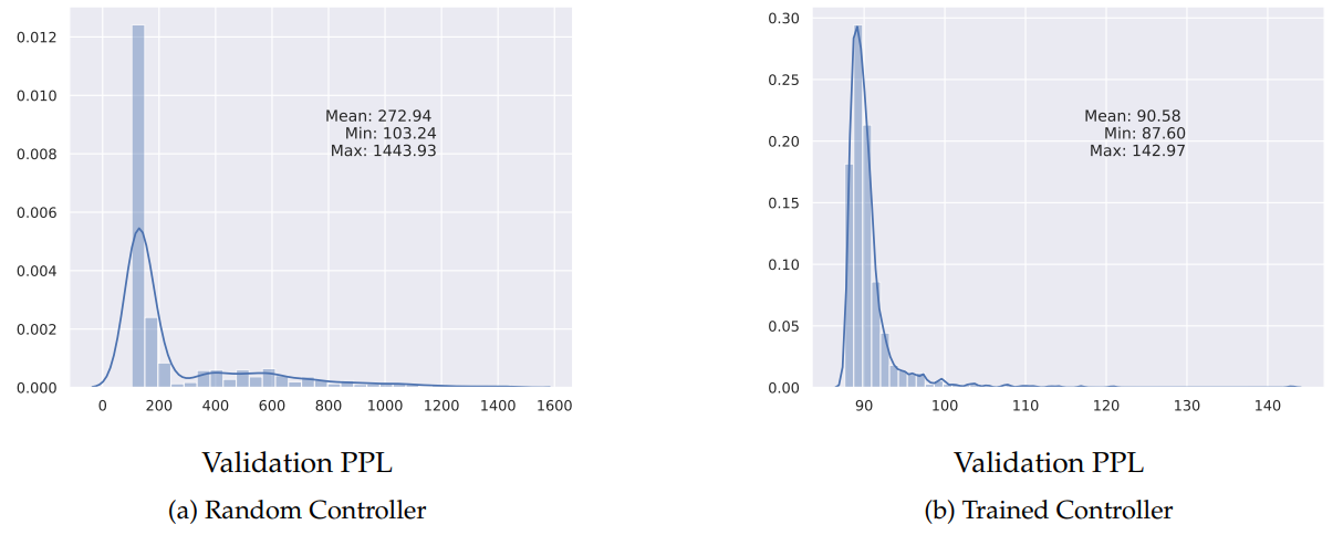
In our experiments, as well as those done in concurrent work by Sciuto et al. and Li and Talwakar, there seems to be litte to no benefit to using the RL-based controller vs random search to explore the space of architectures. We focus on ENAS for the Penn Treebank language modelling task where the goal is to generate a recurrent cell. As seen in the below figure, when sampling 1000 architectures from a trained controller as oppposed to sampling 1000 architectures from an untrained controller, the trained controller does do better, but this can be explained by the weight sharing scheme rather than the controller’s ability to explore the search space. A trained controller samples a less diverse set of architectures, since by definition it has to be biased. This means that when the shared parameters are updated during training, they have to be effective for less architectures. On the other hand, a random controller samples much more varied architectures, so the shared parameters are updated in an attempt to be effective for too many architectures, but do not end up being particularly effective for any given architecture.
What is the Controller Learning?
If using an RL-based controller does not definitively do better than random search, then what is the controller learning? Deep learning has a reputation of resulting in black-box models that are uninterpretable, though for tasks like image classification, object detection, or even segmentation, there are techniques to visualize what features in the input images NNs pay attention to, though the results are to be taken with a grain of salt as illustrated by Adebyo et al.. At minimum, we would expect the recurrent nature of the controller to bias future decisions based on past ones. This does not happen in ENAS. Such unconditional sampling of architecture decisions is troubling since there might be highly effective cells which require particular connection patterns between the nodes, and such patterns cannot be discovered if it is not possible to condition on past decisions.
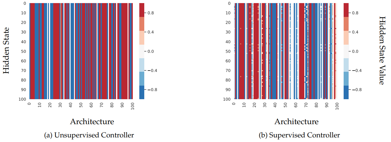
The below figure visualizes the hidden state of the RNN controller for 100 sampled architecture (each row corresponds to the controller hidden state for a single architecture). Notice that in (a), all the rows are the same, even though the sampled architectures are distinct, which demonstrates that the controller does not encode architecture choices in its hidden state.
Is it possible to force memorizing past decisions? We investigate this idea by adding a regularization term to the original loss used to train the controller: a self-supervised objective that requires the controller to be able to reproduce past architectures that it has seen. Specifically,
- After 5 epochs of training, sample and store 1000 architectures per epoch (up to limit of 10, 000). Once this buffer is full randomly replace 100 architectures per epoch
- At the 10th epoch, add a supervised penalty for reconstructing a random sample of 100 architectures from the memory buffer of architectures. This loss is added to the policy gradient loss at each step of controller training: \(\mathcal{L} = \mathcal{L}_{PG} + \mathcal{L}_{Sup}\).
This regularization works similar to how language modelling with RNNs is done in an autoregressive manner: the goal at each time step is to predict what the architecture choice at the next timestep is. There seems to be a bit of a chicken and egg problem here. If we require the controller to reconstruct architectures whose choices at each time step were not conditioned on past time steps in the first place, then are we not just reinforcing that behaviour? In fact, this does not matter since the we are trying to give the controller the ability to memorize and reproduce sequences, and this at least forces that controller’s hidden state to include past choices. (b) in the above figure shows the effect of this regularization, and it is clear that the controller’s hidden state now at least differs between sampled architectures.
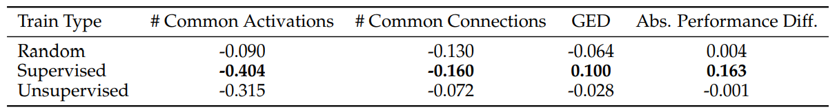
To confirm that this regularization actually makes controller embeddings that provide a meaningful similarity between architectures, we correlated the L2 distance between architecture embeddings and various intuitive notions of architecture similarity such as the number of activation functions, or connections in common between the sampled DAGs. As seen in the below table, the regularization gives the best Spearman correlation, but it’s still quite low. It is likely that a less ad-hoc way enforcing architecture memorization in the controller might help increase correlations even more.
Future Directions
The way in which architectures are currently compared to each other is too simple. Considering just validation set performance leaves out many useful properties that we might want models to have. For example, it might be possible to bias architecture search to generate architectures that are more robust to adversarial perturbations, or architectures that are better suited for pruning. To give architecture search methods this ability, it would be useful to somehow quantify the space of functions that can be learned by a particular architecture. Doing so allows for using more interesting notions of “better” since many architectures give similar validation accuracy, but even if \(A_1\) has slightly worse performance than \(A_2\), maybe it has other properties we value that \(A_2\) does not. With recent interests in the machine learning community such as increasing privacy and reducing bias, smarter architecture search techniques that result in architectures satisfying these requirements are needed.