Introduction
Last summer I had the pleasure of working with a talented undergraduate researcher named Romain Speciel on a project that looked at how to regularize model ensembles in a way that improves robustness to adversarial examples. Our main concern was reducing the transferability of adversarial examples between models as that is a major threat in black-box settings. This article is meant to showcase the work that is further detailed in the preprint, while providing additional intuitions.
We will use \(f\) to refer to a model, and its output should be apparent by context: sometimes it is the predicted label, other times it is the predicted probability. An adversarial example for an image classification model is an image obtained by perturbing an input image in a way that is not noticeable to humans, yet causes the model to misclassify the input. The set of adversarial inputs for a given sample-label pair \(x, y\) is precisely defined as

where \(x\) is the original image, \(\epsilon\) is a positive number selected such that humans cannot tell the difference between the original and perturbed image, and \(p\) is typically chosen to be \(1\), \(2\) or \(\infty\). So in order to find an adversarial input, the following optimization problem has to be solved
This constrained optimization tries to maximize the loss function for a given sample-label pair while also keeping the crafted input x’ close enough to x so that humans cannot differentiate between the two images.
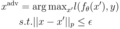
 A classic illustration of an adversarial example for a ResNet-50 model trained on ImageNet
This is not a trivial optimization problem to solve, but we can simplify it by taking the constraint and embedding it into how x’ is crafted. Neural networks are usually trained with some variant of gradient descent as to minimize a desired loss function with respect to model parameters
Similar to optimizing model parameters to fit a dataset (i.e. learning), we can optimize an input by leveraging the differentiability of the model. We use the gradient of the loss with respect to the input image to move in the pixel-space direction that maximizes the loss as follows
where sgn is the signum function which is 1 for positive values, -1 for negative values, and 0 otherwise. By using the signum function, we control the size of the L-∞ norm so that the maximum pixel difference between the perturbed and original image is at most 𝜀. This is known as the fast gradient sign (FGS) attack and is a very efficient way of crafting adversarial examples. However, it is the weakest possible attack, and assumes that the model’s output surface is linear. We note that adversarial perturbations are not unique, and multiple perturbations can exist for a given input, all of which cause a classifier to misclassify it. Additionally, adversarial examples are specific to a given model, though the transferability phenomenon shows that adversarial examples transfer across network architectures, and even model classes.
Importance of Gradients
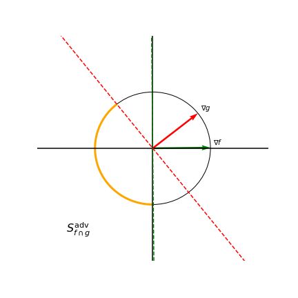
Consider two models \(f\) and \(g\) which have similar accuracy. If the angle between the loss gradient of \(f\) and \(g\) is greater than \(\frac{\pi}{2}\), then perturbing an input \(x\) in the gradient direction of \(f\) will decrease the prediction confidence of \(f\), yet increase the confidence of \(g\). This is best illustrated in subfigure c) of the cover figure for this story where at the base of the red arrows, the model output surfaces intersect and have the same value, while the gradients point in opposite direction. If we can assume that
then in theory an FGS attack could not simultaneously fool both \(f\) and \(g\). Additionally, the disagreement between \(f\) and \(g\), assuming they both have similar test set performance, can be used to flag potential adversarial inputs. This is not a direct defense against adversarial examples, but detection is also important, and having adversarial examples not transfer between models can also decrease attack success rates in black-box settings. Achieving such gradient relationships in practice simply requires the addition of a regularization term to the desired loss function (e.g. cross entropy loss). If the ensemble in question consists of just two models, the optimal regularization term would minimize the cosine similarity
between model gradients. The regularization of gradients is rather abstract, so let’s discuss what this means from the perspective of features used by the models. Orthogonal gradients imply that the models use disjoint feature sets when making classifications such that perturbing the most salient features for model \(f\) has little effect on the predictions of model \(g\). Note that this does not restrict the features that the models use from being correlated. For example, when classifying an image of a car, \(f\) might use tires as a feature, and \(g\) might use doors. Even though these features are likely to co-occur in an image (i.e. the features are correlated), perturbing an image such that \(g\) no longer detects doors in the image will not impact the prediction of \(f\).
Continuing with the car example, gradients with a cosine similarity of less than 0 can be achieved in a scenario where the output of \(f\) increases with the presence of tires, but decreases with the presence of doors, and vice versa for \(g\). In either case, gradient regularization comes at a cost due to models in the ensemble not using the same features, and therefore not being able to achieve maximum performance on an individual basis. There is a fundamental tradeoff between standard accuracy, and accuracy under adversarial perturbations. In cases where there are many features which are weakly correlated with the label yet highly predictive when used together, if those features are not robust, then slight changes to them can significantly change the output.
In practice, a loss function that both optimizes the accuracy of a two model ensemble and regularizes model gradients looks like

The third term regularizes the gradients, and further inspection reveals that it requires second order optimization since we are optimizing gradients rather than parameters.
Measuring Ensemble Cooperation
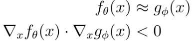
What happens when there are more models involved? Minimizing pairwise cosine similarities between models is no longer enough. Instead, we have to consider the intersection of the adversarial subspaces of all models and regularize model gradients in such a way that minimizes this subspace. Full details can be found in the preprint, so we focus on the motivation behind the approach here, and justify why pairwise cosine similarity is not ideal when considering more than two models as is done by Kariyappa and Quershi. Suppose our ensemble consists of three models. Then maximizing pairwise cosine similarity would result in something close to the blue gradient arrangement below
 Gradient arrangement for three-model ensembles
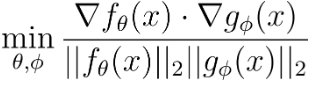
Note how there is only one pairwise angle that maximizes pairwise cosine similarity for three models with 2D gradients, namely \(\frac{\pi}{3}\). However, we don’t need such a strong condition since both the green and yellow gradients visualized would also reduce transferability between models. Our method is able to achieve the less restrictive conditions which makes optimization easier. To further illustrate how model gradients affect the size of an adversarial subspace, the below figure shows the adversarial subspace for a two-model ensemble in orange.
 Adversarial subspace for a two-model ensemble depends on gradients
Any perturbation that lies in the orange region projects negatively onto both the gradients of \(f\) and \(g\), thereby reducing the prediction confidence of both models. To measure how well models within an ensemble cooperate to reduce the adversarial subspace that can simultaneously fool all models, we introduce the Gradient Diversity Rating (GDR):
In short, this rating measures this volume of the adversarial subspace that simultaneously fools all models in an ensemble in the same way (i.e. they all incorrectly predict the same wrong class), normalized by the volume of a unit sphere of the same number of dimensions as models. Have a look at the preprint to see how to minimize GDR for ensembles of varying size. Here we show just the results which indicate that there is a correlation between GDR and adversarial attack success rate, so minimizing GDR is a desirable property of an ensemble.
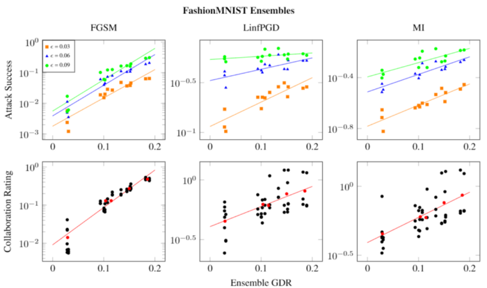 GDR and attack success rate on FashionMNIST
In conclusion, black-box defense settings have better odds of defending against adversaries due to the ability of ML engineers to control model gradients, and create ensembles where attacks do not transfer from one model to another, thereby creating a possible detection mechanism for adversarial examples. There is much more to be understood regarding how generalizable these results are to other datasets, as well as how realistic some of the assumptions are for GDR regularization to be effective. In either case, we believe that this is a worthwhile avenue to pursue, and that the geometric understanding of adversarial examples can result in more principled defense methods.