Introduction
Unpacking the features learned by a deep convolutional neural network (CNN) is a dauting task. Going through each layer to either visualize filters or features scales poorly with network depth, and although some cool figures can be created with this process, the result can be quite abstract, even psychedelic. Techniques such as gradCAM or Guided Backprop get around the need for inspecting individual activations by instead computing which input pixels would cause the largest change in network output if perturbed. As shown by Adebayo et al. back in 2018, some saliency-based model interpretability techniques give results that are too similar to basic edge detection algorithms. For example, Guided Backprop was discovered to produce visualizations that appear to be independent of both model parameters, and data labels.
Today, we explore an alternative to understanding the inner workings of a CNN by creating an interactive visualization that shows the similarity between the features of two images at any given layer of a network. The procedure is simple:
- Perform a forward pass on each image to extract the features at a desired network layer
- Create an invisible grid overlay on each image where the number of cells is equal to the dimension of the extracted features
- Select a grid square from img1 and compute the similarity of that feature to all possible feature locations in img2
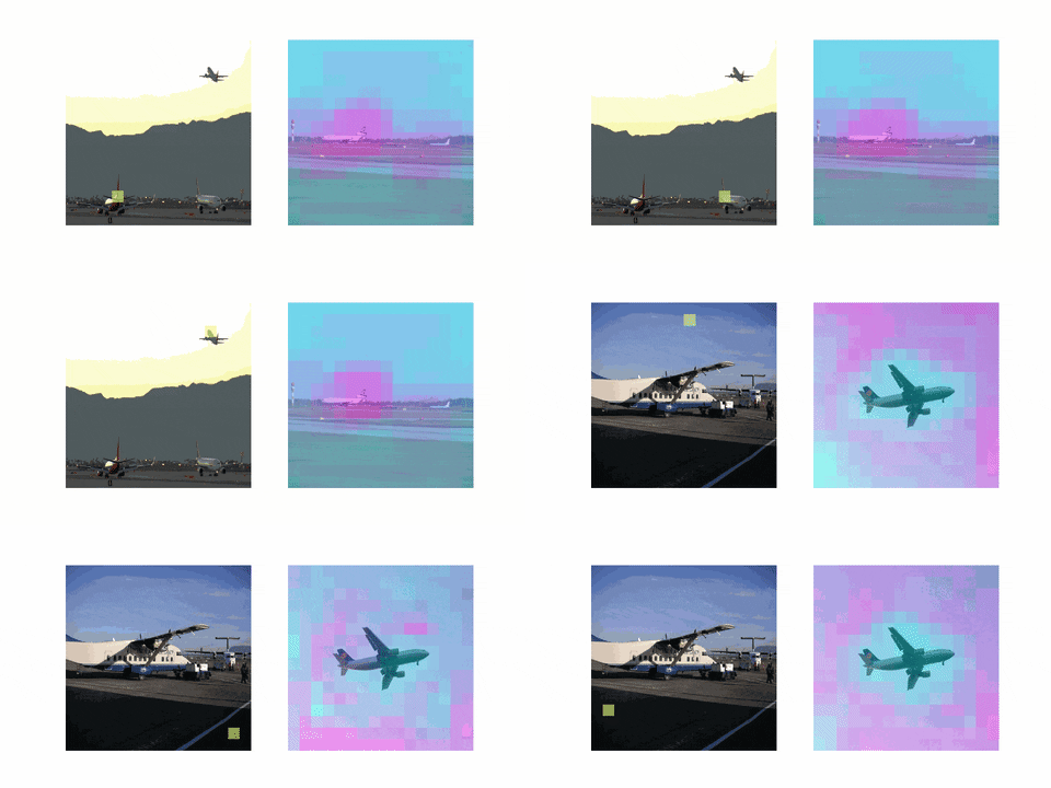
We visualize the procedure on some randomly chosen image pairs from the PASCAL VOC2021 dataset using a ResNet-18 model. The images are resized to be 512x512 pixels using bilinear interpolation. Note that since we are using the 4-th block from this ResNet model, this part of the network downsamples the original resolution by a factor of 32, so we end up with features maps of dimension 16x16. In the left-hand image (img1), the user is able to click on an arbitrary square which gets highlighted yellow. The x and y indices of this square are then used to index the feature map for this image which is just a 512-channel vector. Cosine similarity is used as a similarity metric to compare this feature vector against all 16x16 feature vectors in the feature map for img2.
 Feature similarity heatmap block4 — Images by Everingham et al. from the PASCAL VOC2012 Dataset
The results are somewhat surprising because the receptive field of each neuron in these feature maps is almost the entire image, yet the visualized similarities still depend heavily on location. This suggests that the combination of the learned filters and pooling attenuates the activations to prevent blue sky features from leaking into airplane wing features.
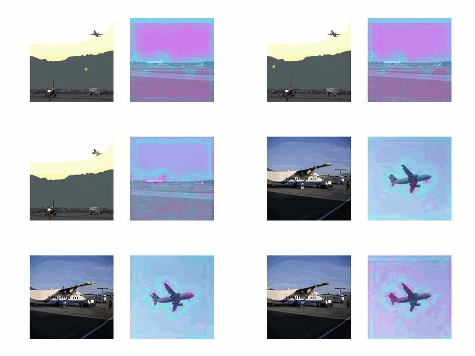
So what conclusions are we to draw from such a visualization? If we look at shallower layers like below where the grid resolution is larger, it becomes apparent that these feature similarities can be used for segmentation purposes:
 Feature similarity heatmap block3 — Images by Everingham et al. from the PASCAL VOC2012 Dataset
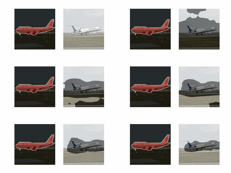
That’s a fun result because the ResNet-18 we’re looking at was trained for image classification, not segmentation. Suppose you have a training image along with a segmentation mask. One could segment a test image by computing the feature similarities of the foreground region from the training image and all possible regions of the test image. Then a threshold could be set via visual inspection to control the IoU of the generated segmentation mask. This task sounds a lot like few-shot semantic segmentation where a model is supposed to generalize to novel objects at test time by propagating feature similarities from images we have masks for to ones which we do not. Let’s see how well this works using features from block 4, this time using a ResNet-50 model:
 Ad hoc segmentation using ResNet-50 block 4 features — Images by Everingham et al. from the PASCAL VOC2012 Dataset
The result is surprisingly good considering that this works right out of the box without any training. At such a low resolution grid of just 16x16, the resulting mask captures too much of the region around the plane, so let’s see if we can fix this by using block 3 features:
 Ad hoc segmentation using ResNet-50 block 3 features — Images by Everingham et al. from the PASCAL VOC2012 Dataset
Sadly, the features in this block do not represent concepts that are high level enough and focus too much on texture as evidenced by the white fuselage of the plane being too similar to the gray sky. This is something that can be fixed by task specific tuning, though that is not the concern of this post.
In an attempt to understand the inner workings of a CNN, we stumbled upon an ad-hoc method that could be used as a baseline for few shot segmentation. We can also use this technique to visualize self-similarities, i.e. using the same image in both the left and right panels to see if a model is learning semantically meaningful features during the course of training. For example, we would expect that foreground object regions in an image are more similar to other foreground regions than to the background. For segmentation, the performance of this technique does not come close to methods that actually train for the segmentation task. However, it does demonstrate that the features learned for classification can be repurposed for segmentation which indicates how powerful and generalizable the feature extraction of deep CNNs is, even without fine-tuning.
