Universal Approximation Theorem - Part 1

Introduction

Early on in my deep learning studies, I heard something along the lines of: neural networks are universal function approximators. This made me really excited about the potential of a correctly specified neural network to fit a dataset, assuming that there does exist a mathematical relationship between the inputs and targets. Don’t get me wrong, this is a fantastic theoretical result, but it needs to be taken with a grain of salt.

The statement I made above is a watered down version of something called the Universal Approximation Theorem (UAT). I won’t repeat it here, but for the sake of completeness I encourage you to take a look at the wikipedia article, as well as this great post. The limitation of the UAT that i want to address in this blog series is that the domain of the function that we are trying to fit has to be covered by our training data. If you read the previous statement a few times while wearing the hat of a pessimist, you’ll notice that the UAT is not what it seems to be on the surface. In fact, a very grim interpreration of the UAT is that neural networks have the ability to overfit the training data with arbitrarily high accuracy.

What’s more interesting is that even a neural network with a single hidden layer that has an arbitrarily large number of hidden units is able to do the above mentioned function approximation. The aim of today’s blog post is to show that this is true in the simplest case: a linear model. Before you get too disappointed, this is just part 1 of a 3-part blog series that is structured as follows:

• Part 1: Introduce UAT and show its power on the most simple function possible
• Part 2: Show how and why a neural network fit to a quadratic function and a sine function fails to generalize
• Part 3: Discuss and try to implement a new neural network layer that might help our model generalize better

Fitting a Linear Function

Let’s begin by defining an arbitrary univariate linear model and train a neural network to learn its weight and bias. The function we will be trying to fit is

Define Imports

import numpy as np
import matplotlib.pyplot as plt
from keras.layers import Input, Dense
from keras.models import Model

Create Data From Function

To keep things gratuitously simple, we won’t even add noise to the data we are trying to fit. For our training data, we will take unformly spaced inputs on the interval \([0, 1]\). For our test data, we will take uniformly spaced inputs on the interval \([53, 60]\). The test data interval doesn’t really matter since given any linear function \(f\), the difference in height for any two pairs of points \((x_{1}, x_{2}), (x_{3}, x_{4})\) will always be the same as long as \(x_{1} - x_{2} = x_{3} - x_{4}\). Notice how this is not true for any polynomial of degree 2 or greater. This is a key point that limits neural networks from generalizing when approximating more complicated functions.

def create_linear_model_data(w, b, n):
    x_train = np.linspace(0, 1, n)
    y_train = (w * x_train) + b
    
    x_test = np.linspace(53, 60, n)
    y_test = (w * x_test) + b
    
    return (x_train, y_train, x_test, y_test)

Define Model

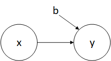
Since we are working with a univariate linear function, our neural network doesn’t even need a hidden layer! This way of framing the problem allows us to learn the actual weight and bias of our model. When we’ll try to fit more complicated functions in part 2 of the blog series, we’ll see how this isn’t possible given the available activation functions, so we’ll have to resort to evaluating those models using just the test data and not the weights fit.

def create_model():
    x = Input(shape=(1,))
    y = Dense(1, activation="linear")(x)
    
    model = Model(x, y)
    model.compile(optimizer="sgd",
                  loss="mean_squared_error", 
                  metrics=["mean_squared_error"])
    
    return model

Train Model

We can now start training the model and see how well it does. It takes about 1000 epochs to converge to the right weight and bias values.

def train_model(x_train, y_train, x_test, y_test, epochs=1000):
    model = create_model()
    
    model.fit(x_train, y_train, epochs=epochs, validation_data=[x_test, y_test])
    
    return model

x_train, y_train, x_test, y_test = create_linear_model_data(3.2, 4.15, 100)
model = train_model(x_train, y_train, x_test, y_test)

Evaluate Model Performance

The way we structured our network allows us to see if it learned the linear function we specified earlier by simply inspecting the weights.

print(model.layers[1].get_weights())

The results I managed to get after 1000 epochs of training are: \(w=3.20200801, b=4.14892197\). This was to be expected since we have a perfectly defined model for a dataset that has no noise.

Another way we will evaluate performance later in part 2 of this series, where there won’t be a correspondence between the weights our model learns and the coefficients of the functions we are trying to fit, is by plotting the predicted values.

def predict_targets(model, x):
    return model.predict(x)

def visualize_predictions(x, y_true, y_pred):
    fig = plt.figure(figsize=(16, 9))
    ax = fig.add_subplot(111)
    ax.plot(x, y_true, c="b", label="True")
    ax.plot(x, y_pred, c="r", label="Predicted")
    ax.legend()
    
    plt.show()

predicted = predict_targets(model, x_test)
visualize_predictions(x_test, y_test, predicted)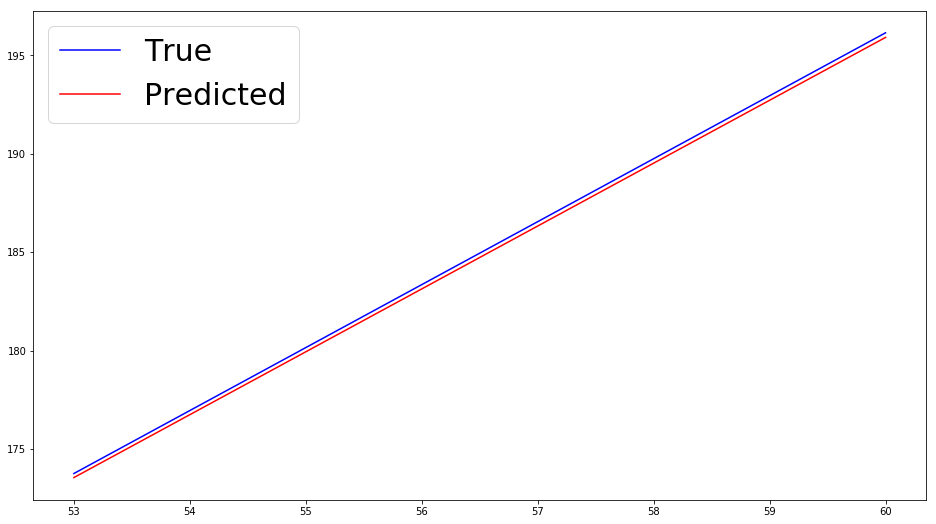

I know that some of you advanced readers were bored to death by this blog post, but it is an essential building block for the more intricate posts to follow. Next time, we will try to fit more advanced functions and see how overfitting comes into play. For now, play around with the code and see how adding noise to the dataset makes it harder for the model to learn the right weights.

Stick around for the more interesting part 2!