Universal Approximation Theorem - Part 2

Introduction

In today’s post, we look at fitting a quartic function. Furthermore, we’re going to take a look at how far away we have to move from our training dataset in order for our predictions to stop being accurate.

Let’s begin by defining the function we will try to fit and highlight the key difference between it and the linear function that we looked at in part 1 of the series.

Fitting A Quartic Function

So what’s so special about a quartic function as opposed to a linear function? Mathematically, the slope of a function in the form

changes as a function of \(x\) as indicated by the first derivative

If we think of what neural networks do at a high level, it’s easy to see why we can’t fit the above function within arbitrary accuracy on an infinite domain. In each layer, a neural network takes linear combinations of the outputs from the previous layers and applies activations to the said linear combinations. What we would need is the ability to take non-linear combinations.

We stick to the UAT and try to fit the following function using a neural network with a single hidden layer and a sigmoid activation function.

Define Imports

import numpy as np
import matplotlib.pyplot as plt

from keras.layers import Input, Dense
from keras.models import Model
from keras.optimizers import Adam

Create Data From Function

Like we did in part 1, we create data without any noise to keep things simple.

def quartic_function(args, x):
    return (args[0] * (x ** 4)) + \
           (args[1] * (x ** 3)) + \
           (args[2] * (x ** 2)) + \
           (args[3] * x) + \
           args[4]

def create_data(train_start, train_end, test_start, test_end, n, f, args):
    x_train = np.linspace(train_start, train_end, n)
    y_train = f(args, x_train)

    x_test = np.linspace(test_start, test_end, n)
    y_test = f(args, x_test)

    return (x_train, y_train, x_test, y_test)

Define Model

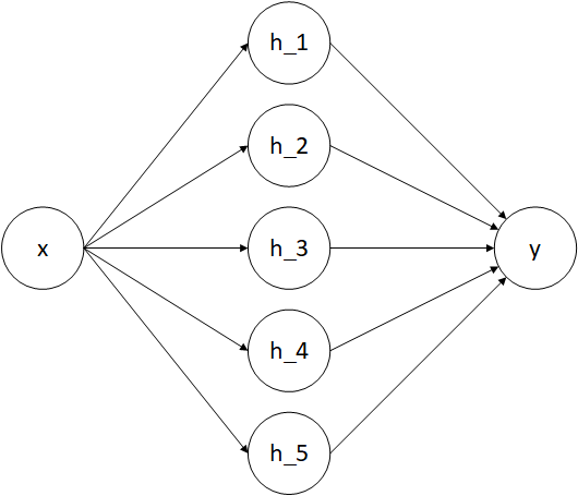
The above diagram shows our model at a high level with activation functions and biases suppressed. As you can see, it only has 5 neurons in the hidden layer! Less neurons might work too, but then it might take longer for the model to converge.

def create_quartic_model():
    x = Input(shape=(1, ))
    
    h = Dense(10, activation="sigmoid")(x)
    
    y = Dense(1, activation="linear")(h)
    
    model = Model(x, y)
    model.compile(optimizer=Adam(lr=0.01),
                 loss="mean_squared_error",
                 metrics=["mean_squared_error"])
    
    return model

Train Model

1000 epochs is enough for a satisfactory fit. Our training data consists of 1000 uniformly spaced points on the interval \([-1.5, 1.5]\). Our test data consists of 1000 uniformly spaced points on the interval \([8, 13]\).

def train(x_train, y_train, x_test, y_test):
    model = create_quartic_model()
    
    model.fit(x_train, y_train, epochs=1000, batch_size=100, validation_data=[x_test, y_test])
    
    return model

x_train, y_train, x_test, y_test = create_data(-1.5, 1.5, 8, 13, 1000, quartic_function, [5, 4, -6, -4, 1])
model = train(x_train, y_train, x_test, y_test)

Evaluate Model Performance

First, we look at how well the model does on the training interval.

def predict_targets(model, x):
    return model.predict(x)

def visualize_predictions(x, y_true, y_pred):
    fig = plt.figure(figsize=(16, 9))
    ax = fig.add_subplot(111)
    ax.plot(x, y_true, c="b", label="True")
    ax.plot(x, y_pred, c="r", label="Predicted")
    ax.legend(loc=2, prop={'size': 30})
    
    plt.show()

predictions = predict_targets(model, x_train)
visualize_predictions(x_train, y_train, predictions)

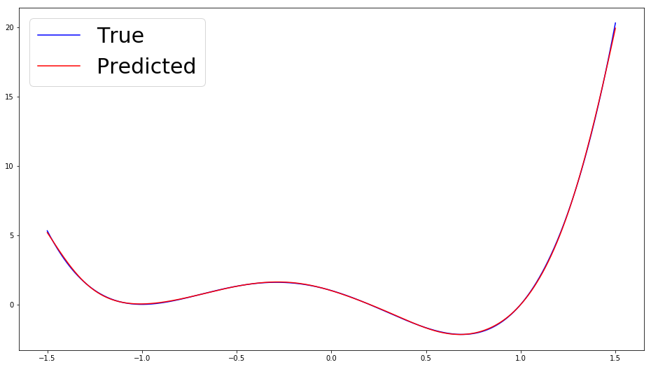
This is close to a near perfect fit, so what’s the issue? Let’s look at how this fit holds as we move farther away from the training interval.

x = np.linspace(-2, 2, 1000)
y = quartic_function([5, 4, -6, -4, 1], x)
predictions = predict_targets(model, x)
visualize_predictions(x, y, predictions)

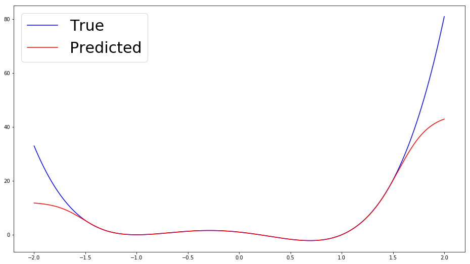
Alas, the overfitting that I was talking about this entire time finally makes an appearance. Let’s consider why this happens. The function is essentially being fit by a linear combination of sigmoid functions. These sigmoid functions are curved enough that a combination of them can be aligned so that they touch our function of interest quite well. However, sigmoid functions plateau as \(x\) moves away from the inflection point, so we get the kind of behaviour seen above where our predictions suddenly stop following the shape of the target function.

Investigating Individual Sigmoids

Now that we know conceptually how the function fitting takes place, let’s make it more concrete by breaking things down and viewing the individual sigmoid functions reponsible for giving us the above fit.

def sigmoid(z):
    return 1 / (1 + np.exp(-z))

sigmoid_params = []
sigmoid_boost = []

for k in range(0, 5):
    weights = model.layers[1].get_weights()
    sigmoid_params.append([weights[0][0, k], weights[1][k]])
    
for k in range(0, 5):
    weights = model.layers[2].get_weights()
    sigmoid_boost.append([weights[0][k, 0], weights[1][0]])

sigmoid_predictions = []

for k in range(0, 5):
    sigmoid_predictions.append(sigmoid(sigmoid_params[k][0] * x + sigmoid_params[k][1]) * sigmoid_boost[k][0] + sigmoid_boost[k][1])

The above code simply extracts the parameters for the sigmoid activation functions learned by the model. We can visualize these sigmoids like so

def visualize_multiple_predictions(x, y_true, ys):
    cmap = plt.get_cmap('plasma')
    colors = cmap(np.linspace(0, 0.8, len(ys)))
    fig = plt.figure(figsize=(16, 9))
    ax = fig.add_subplot(111)
    ax.plot(x, y_true, c="green", label="True")
    
    for i in range(0, len(ys)):
        ax.plot(x, ys[i], color=colors[i], label="Sigmoid" + str(i))
        
    ax.legend(prop={'size': 32})
    
    plt.show()

visualize_multiple_predictions(x, y, sigmoid_predictions)

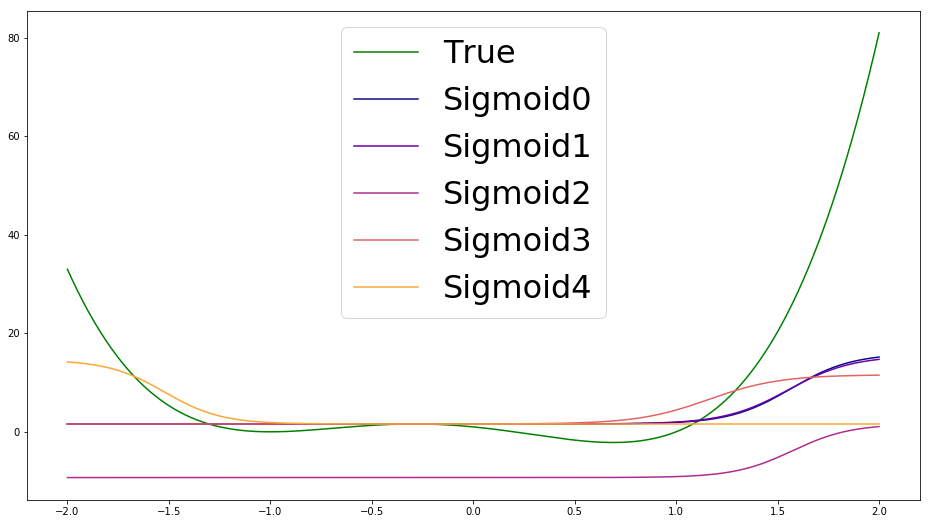
All of these sigmoids are added together to make the overall prediction of our network that was seen earlier. Even though this hasn’t been a rigorous mathematical argument, I hope that this empirical evidence convinces you that neural networks can overfit even very simple datasets without any noise.

Discussion

The question now becomes, is there anything we could do to remedy this? Could we perhaps train longer to get better results? Would a different optimization algorithm be more effective? What if we stack some more layers and use Tanh or ReLU as activation functions instead?

While these questions may be interesting, there’s just one problem: no matter what we do with the architecture of the network, our output layer will end up being a linear combination of some composition of functions that either have a limited range like Tanh or are linear like ReLU. We could add all the regularization and hyperparamter tuning in the world, yet the phenomenon of our predictions deviating from the true function will still happen.

Recall that the UAT only gives us guarantees about being able to fit the function of interest on the interval that contains our training data. If we want our model to make accurate predictions on a larger interval, then our training data needs to have a larger interval as well.

A final cause of overfitting could be that the model we are using has a capacity that is too high. This is highly unlikely considering the number of datapoints (1000) in the training data, and the fact that we only use 5 neurons in the hidden layer.

Next Time

In the final part of this blog series, I’m going to try and make a neural network that can fit the above function with decent accuracy even on an interval that is quite far away from the training interval, so stay tuned!