Introduction
It’s been too long since my last post, so expect to see a chain of new posts in the coming months. Back to the UAT madness that I started looking at last year.
In part 2 we looked at fitting a relatively simple polynomial function using a single hidden layer deep NN. There is something special about fitting polynomial functions that makes them easy to fit: lack of periodicity. I’ll justify this claim later in this post, but for now lets look at how we’ve been representing functions in Python.
By the end of this post, we will be able to fit a sinusoidal function like this one:
numpy Function Representation
When we fit a dataset with any ML technique, we are hostage to the training data. In the case of single-variable function interpolation, we represent a function as a table of \(x\) and \(y\) values. Thus, we are representing continuous mathematical objects with a discrete, limited-precision sample. We do this because it is impossible to collect an infinite amount of training data, and because infinitely many real numbers cannot be represented on digital computers.
Periodicity is Hairy
What does this seemingly harmless drawback of digital computing have to do with fitting periodic functions? It allows for undefined behaviour to occur between the discontinuous samples in our training data! Entertain the following two functions for a moment:
\begin{align} f_{1}(x) = \mathrm{sin}(x) \qquad f_{2}(x) = 18202 \cdot \mathrm{sin}(x) \end{align}
If our ground truth function is \(f_1\) and training data is sampled on the interval \([-5, 5]\) with \(1000\) evenly spaced points, then the \(MSE(f_1, f_2) = \mathrm{8.425e-04}\). This is a scary observation because a function that is so obviously different yields such a small MSE. In other words, the period of \(f_2\) is a local minimum that we can get stuck in, albeit it would take quite a few iterations to move a period initialized near zero to such a large value.
As we’ll see later, extremely bad minima such as this are a reality. Hope is not lost since there are basic techniques we can use to deal with such problems. A basic solution is to incorporate weight decay into our loss function to discourage large period values.
Practical Considerations
Let’s introduce the specific function parameterization that we will be dealing with later on in the code:
\begin{align} f(x) = a \cdot \mathrm{sin}(b \cdot x - c) + d \end{align}
So all we have to do is fit 4 parameters which means that our network will have a single hidden neuron that computes the above function, and we want it to learn the best values of the 4 parameters. This is easier said than done because \(a\) and \(d\) are slightly related, as are \(b\) and \(c\). Allow me to explain what I mean by this.
\(a\) specifies the amplitude while \(d\) specifies the vertical translation. If we consider only the peaks of the sine wave, we can get our initial function to fit the ground truth (minimize MSE) by either shifting it up, or increasing its amplitude as seen below:

The green graph is the ground truth function \(f_{\mathrm{gt}}(x) = 3 \cdot \mathrm{sin} (x)\), the blue graph is \(f_{\mathrm{amp}}(x) = 1.5 \cdot \mathrm{sin} (x)\), and the red graph is \(f_{\mathrm{gt}}(x) = \mathrm{sin} (x) + 2\). This shows how an optimization procedure might get confused between which two parameters to update as they both have a similar effect. A similar confusion is possible for the parameters \(b\) and \(c\).
Before we get into the code, I would be remiss if I didn’t mention this paper by Martius et al. It seems like they have already implemented the idea that I will be covering in this post, and I highly recommend you read their paper because it contains great experiments and looks at neural networks in an unconventional way.
Code
The theory behind fitting a sinusoidal function is not as interesting or complicated as the practical aspect. To overcome the challenges mentioned above, we have to carefully tune hyperparameters. This code section has been written to be self contained such that if you copy all of it into a python file, it should run without any issues. First, we need to define our model, and doing so requires using custom Keras layers. Bear with me as this layer definition is a bit cumbersome, but it isn’t doing anything too fancy. We begin with the imports:
Imports
from keras import backend as k
from keras.initializers import RandomNormal
from keras.layers import Input
from keras.models import Model
from keras.engine.topology import Layer
from keras.regularizers import l2
from keras.optimizers import Adamax

import numpy as np
Custom Layer
class SinusoidalLayer(Layer):
    def __init__(self, output_dim, kernel_intializer=None, kernel_regularizer=None, **kwargs):
        self.output_dim = output_dim
        self.kernel_initializer = kernel_intializer
        self.kernel_regularizer = kernel_regularizer
        super(SinusoidalLayer, self).__init__(**kwargs)

    def build(self, input_shape):
        self.amplitude = self.add_weight(name="amplitude",
                                         shape=(1,),
                                         initializer=self.kernel_initializer,
                                         regularizer=self.kernel_regularizer,
                                         trainable=True)
        self.shift = self.add_weight(name="shift",
                                     shape=(1,),
                                     initializer=self.kernel_initializer,
                                     regularizer=self.kernel_regularizer,
                                     trainable=True)
        self.period = self.add_weight(name="period",
                                      shape=(1, ),
                                      initializer=self.kernel_initializer,
                                      regularizer=self.kernel_regularizer,
                                      trainable=True)
        self.bias = self.add_weight(name="bias",
                                    shape=(1, ),
                                    initializer=self.kernel_initializer,
                                    regularizer=self.kernel_regularizer,
                                    trainable=True)

    def call(self, x):
        return self.amplitude * k.sin(self.period * x - self.shift) + self.bias

    def compute_output_shape(self, input_shape):
        return (input_shape[0], 1)
A few methods here need explaining. build(self, input_shape) just makes keras aware of the 4 parameters that we will be using as part of our function and is similar to generic custom layer definitions like this example. From the shapes of the parameters, it should be obvious that this custom layer conists of just a single neuron.
call(self, x) defines the forward pass through this layer. It simply computes the function \(f(x)\) defined above.
compute_output_shape(self, input_shape) is another mandatory method required by keras and in this case just returns a tuple of shape (batch_size, 1) since the layer has just a single neuron.
Custom Model
The custom model is extremely simple and consists of just an input layer and the custom sinusoidal layer defined above.
def create_periodic_model(stddev=0.01, reg=0.0001):
    x = Input(shape=(1, ))

    y = SinusoidalLayer(1, kernel_intializer=RandomNormal(stddev=stddev), kernel_regularizer=l2(reg), name="sinusoidal")(x)

    model = Model(x, y)

    return model
Training Procedure
The below training procedure is nothing we haven’t seen before. I decided to put it in a for-loop so I could extract the predictions after every epoch for plotting purposes, though there is likely a better way to do that with callbacks. Notice the large learning rate. This is required since if the values of our function parameters are large, it would be pretty much impossible to nudge the randomly initialized values that far. The batch size is also large in relation to the data we’ll be using since we want to avoid the possibility of sampling just peaks or valleys.
def train_basic(model, epochs, x_train, y_train, x_test, y_test):
    model.compile(optimizer=Adamax(lr=5),
                 loss="mean_squared_error",
                 metrics=["mean_squared_error"])
    preds = []

    for i in range(epochs):
        model.fit(x_train, y_train, epochs=10, batch_size=250, validation_data=[x_test, y_test], verbose=False)
        pred = model.predict(x_train)
        preds.append(pred)

    return model, preds
Generating Data
Here is a basic way of generating data for such experiments. It let’s us specify the function of interest, choose training and test set intervals, as well as indicate whether or not we’d like to add noise to the data.
def sin_function(args, x):
    return args[0] * np.sin((args[1] * x) - args[2]) + args[3]


def create_data(train_start, train_end, test_start, test_end, n, f, args, add_noise=True):
    x_train = np.linspace(train_start, train_end, n)
    y_train = f(args, x_train)

    if add_noise:
        y_train = y_train + np.random.normal(scale=0.25, size=y_train.shape)

    x_test = np.linspace(test_start, test_end, n)
    y_test = f(args, x_test)

    if add_noise:
        y_test = y_test + np.random.normal(scale=0.25, size=y_test.shape)

    return (x_train, y_train, x_test, y_test)
Fitting the Data
Time to abuse our hardware and fit the dataset. We generate training data on the interval \([-5, 5]\) and test data on \([-7, 7]\). Mind you, generating test data is not really necessary now that we are using the actual functional form we are interested in as opposed to combinations of arbitrary activation functions.
x_train, y_train, x_test, y_test = create_data(-5, 5, -7, 7, 1000, sin_function, [4, 20, 0.5, 0], add_noise=False)

model = create_periodic_model(0.5, 0.00005)
model, preds = train_basic(model, 250, x_train, y_train, x_test, y_test)
Reproducibility
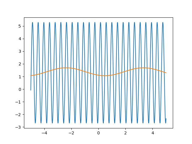
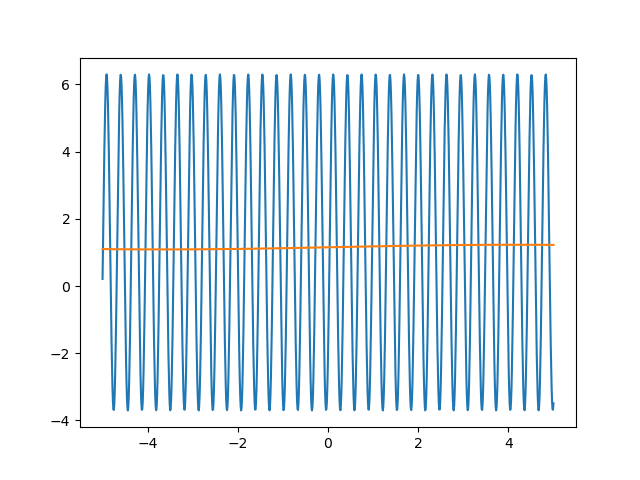
Many machine learning experiments can be difficult to reproduce due to the stochastic nature of optimization procedures. Routine procedures such as shuffling training data or sampling mini-batches can cause a training run to converge in more or less epochs. The experiment in this blog post suffers from the same issues, but it also suffers from an additional issue. The training procedure itself is unstable due to the large learning rate required, so it could take a while for it to converge if it ever does converge. The importance of learning rate is highlighted in the below animations.
 lr=5
lr=5
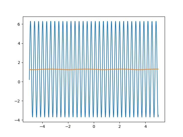 lr=0.75
Conclusion
If you’ve made it to this point, you have fit a sinusoidal function using a neural network via Adamax. This journey of pushing the limits of the UAT has been fun, and we now have a viable solution for function interpolation that can also generalize outside of the training domain. Essentially, we are performing regression using basis functions, and this can be extended to arbitrarily many basis functions by having one neuron per basis fucntion. Stacking layers of such neurons will allow us to fit functions composed of other functions. I’ve run some experiments trying to fit combinations of sinusoidal and polynomial functions, but it seems that the polynomial parameters dominate, and the parameters for the sinusoidal function don’t change much since it is the polynomial component that affects the loss function the most.
I hope you have learned something unconventional about neural networks today, and stay tuned for more wild ideas!